Creating cells & portals
Last Updated November 19, 2013
Simple Z-Buffer Hidden surface removal is unsuitable for processing complex scenes. We need a system to quickly remove objects and polygons from processing if the are not visible in the current frame. We do not want to have to clip every single polygon in a scene comprising millions of faces.
Z-Buffer Deficiencies
We will create a structure to organise the elements of a scene in such a way to allow efficient visibility processing. Most scenes are characterized by having relatively few objects, but the objects are composed of many polygons. To be efficient these structures will subdivide the scene down to individual polygons.
Efficient Visibility processing has two main goals
Note: Testing if an object lies inside or outside a view frustum is a form of collision detection, and the techniques discussed here can be adapted to collision detection.
The structures created to perform visibility processing are generally divided into two types;
These structures are normally very expensive to generate, so are usually pre-computed in a once-off operation.
Spatial Subdivision involves dividing space into a number of regions and labeling these regions with object occupancy. The success of such schemes depends on how finely we divide space.
A simple spatial subdivision is into regular voxels. (A voxel is the 3D equivalent of a pixel). Space can be divided in to a regular grid of cubes. Each cube can be labeled as empty or occupied by objects.
A visibility algorithm could determine which voxels lie inside the view frustum and then process objects belonging to those voxels.
A voxel based system has a major drawbacks;
Most scenes consist largely of empty space (consider a room or a landscape). Typically most (>90%) of the voxels will be empty. There exist more advanced schemes which take a more efficient approach to structuring space (Octrees & BSP).
In order to efficiently apply frustum culling and occlusion culling to a terrain patch, the rectangular patch is recursively subdivided into smaller and smaller rectangles. The amount of subdivision is controlled to achieve a balance wherein the granularity is small enough for the culling algorithms to be effective, but not so small that the number of rectangles becomes unmanageably large.
To organize the pieces of the terrain patch, a quadtree is used. This is simply a tree in which each node has four children. The root node of the quadtree contains the entire terrain patch. Successively lower levels of the quadtree contain smaller portions of the terrain patch. The leaves of the tree then contain the individual rectangles produced by the last level of subdivision.
Organizing terrain into a quadtree is useful because it allows efficient application of frustum and occlusion culling. To apply frustum culling to a quadtree, for example, one first tests the root node against the viewing frustum. If the root node is completely within the frustum it can be accepted and drawn immediately; if it is completely outside the frustum, it is rejected. If the node is partially inside and partially outside the frustum, as is evidently the more common case, it is subdivided into its four children and the process is repeated with each. The following pseudocode illustrates this algorithm:
  add root_node to queue;
  while (queue is not empty) {
  pop node off queue;
  if (node is completely inside frustum)
  	accept node;
  else if (node is completely outside frustum)
  	reject node;
  else // Node must be partially inside, partially outside
  	for each child of node
  		add child to queue;
  }
Octrees subdivide space in a hierarchical manner. The approach proceeds as follows;
Note that the interior of an object is considered empty space. Only surfaces count as 'objects'
The generated set of cubes can be efficiently stored in a tree whose node have at most 8 branches (hence the name OCTree).
There will be two types of terminal nodes in the tree, some nodes correspond to regions of empty space, other nodes will be nodes of minimum size and contain part or all of an object.
This structure provides an representation of the entire scene and at high resolution will require an enormous amount of storage.
An alternative subdivision provides a representation of the distribution of objects in the scene. In this case we subdivide a region only if it contains more than one object.
Octrees (& BSP trees) take advantage of the concept of coherence. Coherence is a very important idea in computer graphics, simply states that an entity (location in space, pixel, point in a line, polygon, piece of carpet, person etc.) is likely to be very similar to its neighboring entities.
A binary space partioning tree, as the name suggests divides each region of space into two sub regions, but the most important difference between BSP trees and Octrees, is that while octrees use a planes on regular grid to determine subdivision, BSP trees can use planes of any orientation and normally the planes used are defined by the faces in the scene. This kind of scheme is often called adaptive partitioning as the partitioning adapts to the actual distribution of objects rather than a regular grid.
A plane divides space in to two regions, technically one of these regions is positive (above the plane) and the other is negative (below the plane). To create a BSP tree, we will use planes to successively divide space.
First choose a plane A to divide space (we will examine strategies later for how to choose A and other planes). A will be the root of our tree and will have two branches representing the positive half-space and the negative half-space. Any objects in the positive half space will ultimately end up in the right half of the tree and objects in the negative half-space will end up in the left half of the tree.
This process continues recursively. we choose a plane B to subdivide the negative half space, B becomes the root of a A's left sub-tree. We also choose a plane C to subdivide the positive half-space.
This process continues until a half space contains only one object and the object becomes a leaf of the tree.
Having constructed a tree (usually a once off operation, done at the build stage), we can now construct a visibility ordering (order all the objects in the scene from nearest to the camera to furthest).
Find the node corresponding to the position of the camera, that object is 'closest' to the camera, the next closest object is the node's sibling, to retrieve the remaining nodes, we must ascend to the next level and traverse the remaining nodes.
In this case 'closest' means that there can be no intervening objects.
Check Out this BSP applet
To generate a visibility order from the BSP tree, follow these steps;
This produces a near to far ordering, but swapping steps 3 & 5 will produce a far to near ordering.
drawbsptree(node){

	if(plane intersects viewvolume){
		if(distanceA is positive){ // distance from the VP to the plane
			drawbsptree(node.right)
			render(node.face)
			drawbsptree(node.left)
		}
		else{//distanceA is negative
			drawbsptree(node.left)
			render(node.face)
			drawbsptree(node.right)
		}
	}
	else
	//current plane outside viewvolume
	//therfore everthing on the far side is not visible
	// so need only traverse one subtree
	{
		if(distanceA<0)
			drawbsptree(node.left)
		else
			drawbsptree(node.right)
		render(node.face)
	}
}
Early rendering methods used the Painters algorithm to draw visible polygons. Polygons painted in far-to-near ordering. The nearer face simply drawn over the further faces. This is inefficient as rendered polygons are drawn over and the effort to calculate the lighting was wasted.
A more efficient way is to draw the faces is near-to-far, but obviously we need some way to mark which pixels have been written to. To do this we maintain a stencil buffer which records which pixels have been draw and which have not. Drawing can stop when all the pixels in the stencil buffer have been painted.
Use of the BSP tree solves another problem associated with the simple painters algorithm which does not work for intersecting polygons. BSP splits these polygons, which removes the problem.
However transparency effects are much easier to implement with a far-to-near ordering.
Choosing appropriate separating planes can be a difficult problem, and for a scene with n objects we need to choose from n2 planes. For a polygon based scene we can choose our partioning planes containing face polygons. Is is likely that some partioning planes will intersect face polygons. In this case the face will have to be split into two constituents.
The approach to building this tree is recursive;
Determineing whether a point is on the negative or positive side of the face, is a matter of evaluating the Cosine of angle between a vector from the point to the plane and the plane normal, q is a point on the plane;
n.(p-q) =?
if this expression is less than zero, the angle between the vectors is greater than 90 degrees, therefore the point is 'behind', or 'inside' the plane. This expression can be further simplified;
n.(p-q) =n.p-n.q
n.q is constant for any plane, rewrite as 'd'
n.p-d=?
rewrite n=(a b c), and p=( x y z)
ax+by+cz-d=?
all points who evaluate this expression to zero lie on the plane;
ax+by+cz+d=0 ;point on plane
ax+by+cz+d<0 ;point below plane
ax+by+cz+d>0 ;point above plane
To avoid the expense of splitting a plane in two dimensions, it is normally more expedient to simply add the plane to both sides of the tree, this saves the problem of recomputing texture and light map coordinates.
Backface culling can be performed at no cost during tree traversal. Whenever the viewpoint is in the negative half-space of a polygon, that polygon can be culled.
BSP can cull against the view frustum. A subtree can be culled in one operation if it can be show that the node plane does not intersect the view frustum, the the 'far' side of the plane will not be visible.
For a finite view frustum (i.e. one with a far plane), a far side BSP tree node can be culled(and all its sub trees) if all 5 points of the view frustum lie on the other side of the partition plane.
A BSP tree has two major attributes, which affect how well it performs is various application;
These factors have different importance depending on application.
For simple visible surface determination, every node is visited, so it is important to keep the size down. For collision detection, ray tracing or other processes which 'search' the tree, balance is the key of efficiency.
One method to control the size and shape is to choose a number of candidate polygons (~100) for each partition, and determining the number of splits required (within the same subspace) and the number of polygons on either side. A weighed sum of these measures is calculated for the candidates and the best one chosen. The weights will depend on the application.
For room type environments, it is best to use the walls/floors as partition faces before subdividing room interiors. A typical approach is to process the faces at the periphery first and work your way to the center. Larger polygons, representing walls are unlikely to intersect objects within a room.
For landscapes the terrain is normally build over a regular grid, in this case partitioning should be done on planes perpendicular to the ground plane and aligned with the x or y-axis.
Occlusion culling (OC) or visible surface determination (VSD) is the process of determining which parts of the scene are not visible because although they are inside the view volume, the are occluded from view by other opaque objects, closer to the viewer. Objects that are occluded can be culled from rendering.
This problems is traditionally solved by a HSR techniques such as z-buffer, but the need to examine every polygon maked these techniques inefficient. We will look at some techniques which can remove large numbers of occluded objects quickly.
There's a big difference between occlusion culling and z-buffer rejection. Occlusion query rejects polygons at the geometry level, whereas buffer occurs at the rasterization level. Plus, culling geometry through occlusion query requires more control from the application.
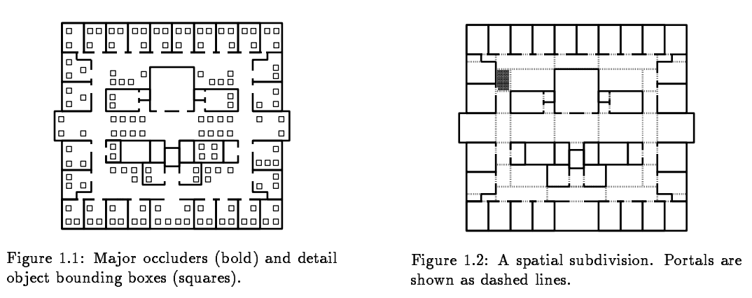
Portals are used to cull objects which cannot possibly be seen from a viewpoint due to nearby walls. Portals are primarily used for interior environments.
A portal is a polygon through which another 'space' is visible (door, corridor, window, tear in space-time continum).
The model database devided into occluders (walls, floors & cielings) and detal objects (everything else). The occluders are used to divide the world into convex 'cells'. This is a spatial subdivision. Portals are constructed where neigbouring cells which are joined by a transparent boundary.
The detail objects for each cell are then enumerated.
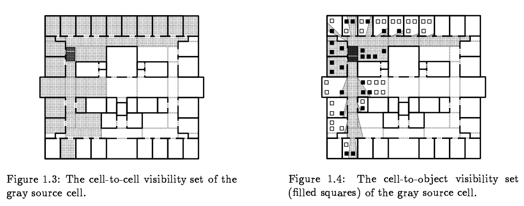
The problem is the reduced to that of determining visibility of objects in the room and objects in adjoining room (and objects in rooms adjoining the adjoining rooms, ...).
Generally, visibility between rooms will be limited, since the occluders will obsure space in adjioning cells. A generalised observer is an abstract observer, free to move anywhere in a cell and look in any direction. A generalised observer may see into a neighbouring cell only through a portal, and into a more distant cell through a portal sequence. These sequences significantly limit the observers visibility.
A cell is visibile from another cell if there exisits a sightline between the two cells which does not intersect an occluder. Using sightlines, a cell to cell visibility set can be generated
For the viewpoint room, objects are culled against the view frustum as normal and visible objects added to the render list. If the view volume intersects a portal, then a new view volume is constructed from the viewpoint and corners of the portal (after the portal is clipped to the old view-volume). The contents of the new room are culled against the new view volume. If the new view volume intersects another portal, the process continues (recursively).
Occluders are a little like the opposite of portals and are typically used in outdoor environments. An occluder is a "bounded" box which lies entirely inside some other large game object (like a building or a mountain). Again a view frustum is created from the camera position and the occluder, with the position of the occluder acting as the near plane.
Any objects inside the main view frustm, and inside the occlusion frustum are not visible. Again, an octree or bsp tree can be used to cull away these objects
Potentially Visible Sets are used to accelerate the rendering of 3D environments. This is a form of occlusion culling, whereby a candidate set of potentially visible polygons are pre-computed, then indexed at run-time in order to quickly obtain an estimate of the visible geometry.
In order to make this association, the camera view-space (the set of points from which the camera can render an image) is typically subdivided into (usually convex) regions and a PVS is computed for each region.
View frustum culling is usually applied to the visible set for a given location .
Moving objects can disrupt the integrity of a BSP tree. A number of methods have been developed to deal with dynamic objects.
The most flexible system is to update the tree as object moves around. The basic approach is to 'delete' an object that has moved, and reinsert the object at its new position.
Insertion is relatively easy, just traverse the tree to find the leaf node 'nearest' to the object and stick the object there.
Deleting a node can result in three trees, merging the three trees can be difficult.
There are 3 types of node removal;
//Initial step: mark all polygons of moved object as "delete"
///////////////////////////////////////////////

Restore(tree){
	if tree.empty retun null;
	if (tree.root is not marked "delete"){
		tree.left=Restore(tree.left) 	// tidy up left sub tree
		tree.right=Restore(tree.right) // tidy up right sub tree
		return tree;
	}
	else{// root is marked for deletion
		if (only one child){
			chlld= Restore(non-empty child)

			replace this node with child
			return child;
		}
		else{// two-non empty children
			child=Restore(larger child)
			replace this node with child
			InsertPolygonsintotree(polygons of smaller tree, larger child)
			return child
		}
	}
}


Benefits
When a target object is moved, the restore function is only relevant for the
  first movement. After the object is deleted from the tree, its nodes are removed
  and reinserted, either as a leaf node or as a subtree of nodes shared with other
  polygons in the object. In this case only the simple (first type) of node removal
  is required. All further movements of the object will result in deletion of
  leaf nodes.
All objects that are likely to be moved should be inserted into the tree last
  of all.
An enhancement to this process would be to leave in place 'deleted' node whose
  sub trees are too large. Nodes with large sub trees are, by definition, not
  common. Leaving them in place (marked as deleted) would prevent having to re-process
  large subtrees.


© Ken Power 2011