Hidden Surface Removal (HSR)

Last updated 5 March, 2008

We have looked at removing backfaces, this stage will usually eliminate about half of the surfaces in a scene from further processing. Once the polygons to be displayed have been clipped, we need to draw themon to the display device (Rasterization).

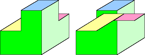
We also need to remove parts of those surfaces that are partially obscured by other surfaces. These are called hidden surfaces. If hidden surfaces are not dealt with correctly, then we may get distorted images like the right of the image below. Rasterization and HSR are usually combined in to a single phase of the rendering pipeline.

Scanline Triangle Filling

This technique fills polygons one scan-line at a time. For each scan-line in the window, we must determine which polygons the scan-line intersects. Because this method draws the polygon scan-line by scan-line, some pre-processing of the polygon mesh is required before rasterization;

Horizontal Edges must be removed, these edges will be drawn when the adjacent edges are processed.

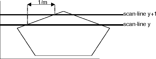
The scan-line method takes advantage of edge coherence, i.e.

Many edges that are intersected by scan-line y are also intersected by scan-line y+1 .
The x-value of the point of scan-line intersection migrates predictably from scan-line to scan-line. The x co-ordinate of the intersection of an edge with a scan-line increases by \frac{1}{m} for each scan-line, where m is the slope of the edge.

An important component in the data structure needed for this algorithm is the edge node. Each edge in the polygon is represented by an edge node. An edge node contains the following information;

y_{upper} , the y co-ordinate of the upper end-point of the edge.
x_{int} , the x co-ordinate of the lower end-point of the edge. As the algorithm progresses, this field will store the x co-ordinate of the point of intersection of the scan-line.
y_{m} , the reciprocal of the slope of the line ( \textstyle\frac{1}{m} ).

We also need an Active Edge List (AEL) which contains the two edge nodes with the lowest y_{lower} . The AEL represent the two edges intersected by the current scan line. The AEL needs to be maintained as we move from on scan-line ( y ) to the next scan-line ( y+1 );

One or both of the edges in the AEL will no longer be intersected by (y+1) . Remove the edges from the AEL, where y_{upper} is less than y+1 .
The intersection point of the scan line with the remaining edges will change for the new scan-line. x_{int} is updated to x_{int} + y_{m} . Note that x_{int} must be stored as a real number to avoid round-off errors.
If the AEL has only one edge, add the remaining triangle edge
Fill the pixels from the x_{int} of one edge to the x_{int} of the next.
Repeat until the AEL is empty.

Heedless Painters Algorithm

This is a very simple but naive algorithm. Find the face with the deepest vertex (vertex with greatest z co-ordinate), and draw that face. Then draw then next nearest face, if two faces overlap, then the most recently drawn face will obscure the first one. This method does not work when faces intersect. The method is very expensive when there is a lot of overdraw in the scene.

Occlusion Buffer (Z-culling)

Occlusion buffer is a refined variation on a reverse heedless painter technique. The method sorts and draws the polygons in a near-to-far order. As pixels are drawn, each pixel is marked as "filled" in an occlusion buffer. The occlusion buffer is a boolean array of the same size as the refresh buffer, initialised as "unfilled".

Before rendering a pixel of a polygon, the occlusion buffer is check to see if the corresponding screen pixel is already filled. If that screen pixel has already been filled, the polygon pixel can be eliminated, otherwise it is draw and the occlusion buffer updated.

This technique is very cost effective where there is a lot of overdraw and lighting or texturing calculations are expensive. Time consuming pixel shaders are not executed for pixels which are never seen.

The demerits of this technique are

the polygons need to be sorted in near to far ordering from the camera
intersecting polygons need to be split to avoid overlap
memory space is used for an occlusion buffer (not important on modern systems)

Depth Buffer Method (Z Buffer)

This is the technique use in most modern rendering systems.

This algorithm tests the visibility of a surface one pixel at a time. For each pixel position (x,y) on the viewplane, the surface with the smallest z co-ordinate (pseudo depth) at that position is the visible surface. So the pixel is drawn with the colour of the closest surface.

Before processing the overall projection matrix M_{tot} has been applied to all the vertices in the model. Two buffers are required for this algorithm. A depth buffer is used to store z-values for each (x,y) pixel position of the scene. And a refresh bufferis used to store colour (intensity) of each pixel position.

Initially all positions in the depth buffer are set to 1 (Maximum depth) and the refresh buffer is filled with background colour.

Each polygon in the model is processed one scan line at a time, and the depth (z co-ordinate) is calculated at each pixel position \textstyle (x,y). The calculated z-value is compared to the value previously stored in the depth buffer at that position. If the z-value is less that the value in the depth buffer, this means that the current polygon is the closest polygon so far observed at that pixel position, the refresh buffer at that position is then filled with the colour of that polygon. Once all the polygons have been processed the refresh buffer should contain a realistic view of the scene, with closer faces correctly overlapping faces that are further away.

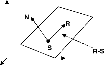
The key to this algorithm is being able to accurately and quickly calculate the depth of a polygon at various points on its surface. We already know the relative depth of the vertices (these have been normalized), but if faces are at an angle to the view plane, we will need some method to calculate the depth of points on the face. To calculate depth we will use the point normalform of a plane. This can be specified by giving a point S(s_{x},s_{y},s_{z}) on the plane and a normal, \vec{\mathbf{N}}, to the plane. For another arbitrary point on the plane \vec{\mathbf{R}}, we know that \vec{\mathbf{N}} is perpendicular to the vector (\mbox{$\vec{\mathbf{R}}$}-\mbox{$\vec{\mathbf{S}}$}) which lies on the plane. This gives us an equation for a plane called the point normal form.

\\ \vec{\mathbf{N}}.(\vec{\mathbf{R}}-\vec{\mathbf{S}})=0 \\ \vec{\mathbf{N}}.\vec{\mathbf{R}}-\vec{\mathbf{N}}.\vec{\mathbf{S}}=0 \\ \vec{\mathbf{N}}.\vec{\mathbf{R}}=\vec{\mathbf{N}}.\vec{\mathbf{S}}

i.e. All points on a plane have the same dot product with the normal to the plane. If we write \vec{\mathbf{R}} (arbitrary point) as $(x,y,z)$ and \vec{\mathbf{N}} .\vec{\mathbf{S}} as a constant D we get;

\vec{\mathbf{N}}\cdot(x,y,z)=D

Expanding the dot product:

n_{x}x+n_{y}y+n_{z}z=D

(which can be re-written as the usual form of a plane: ax+by+cz=D re-arranging we get an expression for the depth at some point (x,y);

\begin z(x,y)=\frac{D-n_{x}x-n_{y}y}{n_{z}} \end

As we process a scan line, the y co-ords stay the same, and the x co-ord changes by one. So if the depth of at position (x,y) has been determined to be z, the depth at the subsequent pixel (x+1,y), z' is;

z'(x,y)=\frac{D-n_{x}(x+1)-n_{y}y}{n_{z}}=z-\frac{n_{x}}{n_{z}}

So we can calculate the depth of the next pixel by adding a constant to the depth of the current pixel. We can calculate the normal for each face by using Newell's method, or by finding two non-collinear vectors on the surface of the face and calculating their cross product.

The Depth buffer is easy to implement, quick and requires no sorting but requires large amounts of memory for the buffers, and depth calculations need to be made at every (pixel)point on every face.

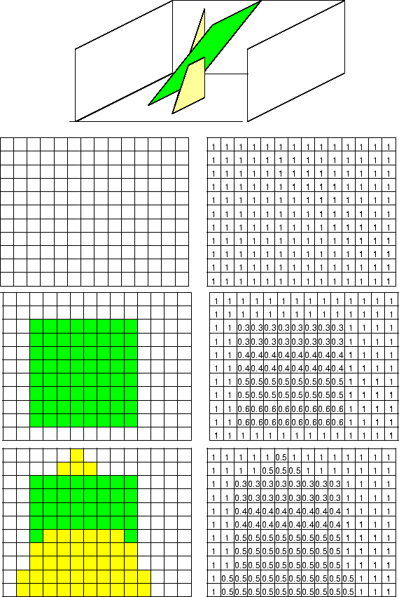
The Scan-Line Method

This HSR technique processes the scene one scan-line at a time. For each scan-line in the window, we must determine which polygons the scan-line intersects. Then for each pixel along the scan line, determine which polygon is nearest the eye at that point; this then determines the colour of that pixel.

Because the scan-line method draws the image scan-line by scan-line, some pre-processing of the polygon mesh is required before rasterization.

Horizontal Edges must be removed, these edges will be drawn when the adjacent edges are processed.
The algorithm uses edge crossing to detect entry and exits of polygons. Each edge crossed changes the "inside-outside parity" When a scan-line passes through the end-point of an edge, it produces two intersections, one for each edge that meets at that vertex. This is OK if the vertex is a local minimum or maximum. If the vertex is not a local extremum, the two intersections will cause the parity to be unchanged. To resolve this problem, when an intersection is not an extremum, simply reduce the y_{upper} co-ordinate of the lower line segment by 1. This will not effect the accuracy of the method as we will use to slope of the line segment before shortening.

To keep track of which polygons we are currently drawing we need to build an edge table, which contains an entry for each scan-line, this entry is a list of all edges first intersected by a given scan line. Each edge contains some information about the edge and a list of associated faces (polygons).

We also need an Active Edge List (AEL) which contains a list of edge nodes. The AEL represent edges intersected by the current scan line. The AEL needs to be maintained as we move from on scan-line ( y) to the next scan-line ( y+1);

Some of the edges in the AEL will no longer be intersected by (y+1). Remove all edges from the AEL, where y_{upper} is less than y+1.
The intersection point of the scan line with the remaining edges will change for the new scan-line. x_{int} is updated to x_{int} + y_{m}. Note that x_{int} must be stored as a real number to avoid round-off errors.
New edges may need to be added to the AEL. If y+1 is equal to y_{lower} of any edges in the edge table, then those edges must be added to the AEL.
The node in the AEL must be stored (for parity checking) in ascending order of x_{int}, so, after adding new edges and updating the x_{int} values of the edges, the AEL must be sorted.

For each polygon in the scene, we maintain a flag which is set IN or OUT depending on whether we are inside or outside that polygon. As we process a scan line, we will cross edges, as we cross an edge we must 'reset' the flag for each polygon which shares that edge. If we are IN a polygon and we pass an edge of that polygon we must reset the flag to OUT. 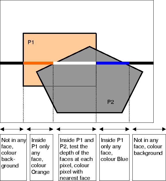As we process a scan-line, pixel by pixel, we need to colour the pixels as follows.

If no flags are set to IN then the pixel gets background colour.
If only ONE flag is set to IN, the pixel gets the colour of face we are in.
If more than one flag is IN, we need to determine which face is closest at that point by calculating the depth of each face as in the Depth Buffer method. The pixel gets the colour of closest face.

When we are IN two or more polygons, we can calculate the closest face for each pixel or we can assume that the closest face at the first pixel of the overlap will remain the closest face until we meet another edge. This way we need only calculate depths at the beginning of an overlap area and need not do the calculations for every pixel. This will allow us to implement a very efficient algorithm, which fills pixel runs between edges. However this optimization will not work for some scenes.