Effect of lighting model (left to right);
Wireframe, Faces Colored (with wireframe), Faces Colored (without
wireframe), lighting model applied (flat shading).
Last Updated April 23, 2008
Realistic views of scenes are obtained by generating perspective projections with hidden surfaces removed and appropriate lighting and colouring applied to the model. A Shading model is used to calculate the intensity of light(colour) we should see when we view the surface. The exact colour of a surface when viewed depends on more than pigmentation; the amount of light striking the surface, the colour of the light, the angle the light strikes the surface, the orientation of the viewer and the texture of the surface all contribute to the actual colour we see (figs below). When we view an object what we see is light from light sources reflected from the surface. There are two basic types of light sources;
In a scene, illumination from light emitting sources is reflected off multiple surfaces, these reflections combine to produce a uniform illumination called ambient light. Ambient light appears to come equally from all directions.

Light emitting sources come in two basic types;
When light strikes a surface, most of it is scattered equally in all directions (figure below). This is called Diffuse reflection. The amount of diffuse reflection from a surface is primarily determined by the roughness or texture of the surface.
If a surface is exposed only to ambient light then we can express the intensity of diffuse reflection as:
(where R_{d} = Co-efficient of reflection of the surface (constant for a given surface (0<=Rd<=1), I_{a} is the intensity of Ambient light).
The level of diffuse reflection of ambient light is similar in all directions. Highly reflective surfaces (smooth or polished) have a R_{d} near one, which means that almost all the incident light is reflected.
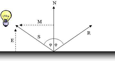
More realistic shading models will include illumination from light sources as well as ambient light. The calculation of diffuse reflection from a point source is based on Lambert's cosine law, which states that the intensity of reflected light is dependant on on the angle of illumination. When a surface is at a steep angle to the light rays, less light strikes the surface (figure below).
To simplify calculations we will assume that the light rays are parallel as they strike the surface (This is a good approximation for sources which are reasonably far away from the surface). We will describe the orientation of a surface with a unit normal vector \vec{\mathbf{N}} and the direction of the light source is the unit vector \vec{\mathbf{S}}.
The angle between the two vectors, \theta, is called the angle of incidence. Lambert's law states that the amount of reflected light is proportional to the cosine of the angle of incidence. This can also be written as a dot product;
A surface is illuminated by a light source only if the angle of incidence is between 0^{\circ} and 90^{\circ}.
Putting all of this together, we get the following equation for the intensity of diffuse reflection due to a directional light source source:
These equations assume we are dealing with mono-chromatic (white) light. In real world situations, light sources have different colors, and our model should be able to handle this. To accommodate the use of colours, our light intensity values and our reflectivity constants should become 3-Vectors, each vector contains values for the Red, Green and Blue components of the light source.
Now I_{s} becomes the 3-vector (I_{sr},I_{sg},I_{sb}) and R_{d} becomes ( R_{dr},R_{dg},R_{db}) where I_{sr} represents the amount of red light in the source and so on. This breakdown is important as different surfaces reflect the colours by different amount; e.g. A surface with yellow pigmentation will reflect a lot of Red and Green, but will absorb most of the Blue light.
When viewing a shiny surface in the presence of a light source, bright spots on the surface are often seen. This is called specular reflection.
Specular reflection is only observed at certain viewing angles and depends on the orientation of the surfae with respect to the viewer and to the light source. On a shiny surface, much of the incident light is reflected away from the surface at an angle similar to the angle of incidence. For real surfaces, specular reflection is observed over a small range of angles around the angle of reflection. As the viewer moves away from the angle of reflection, the specular component decreases.
In figure below,\vec{\mathbf{V}} is a unit vector in the direction of the viewer and \vec{\mathbf{R}} is a vector along the angle of reflection. When \vec{\mathbf{V}} and \vec{\mathbf{R}} coincide, the viewer sees maximum specular refection, as \phi increases, the specular reflection decreases. For shiny surfaces the specular reflection is very bright but visible only over a small range of angles, for less shiny surfaces, the specular reflection is not as bright, but is visible over a wide range of angles. A good approximation to the observed behavior of specular reflection is the Phong Specular Model.
In the Phong model, the intensity of specular reflection is proportional to \cos^{f}(\phi), where f depends on the surface and ranges between 1 and 200. Very shiny surfaces have high values of f, as specular refection is exhibited over a small range of \phi. We know that cos(\phi)=\vec{\mathbf{R}}.\vec{\mathbf{V}}.
(I_{sp}= intensity of specular reflection, R_{s}= co-efficient of specular reflection; R_{s} is usually = R_{d}).
There now remains the question of calculating \vec{\mathbf{R}};
From the diagram above, we can see that the reflection vector is calculated as;
Polygon mesh models are distinguished by the fact that the model only approximates the actual objects represented. A Shading model must apply some reflection model (e.g. Phong reflection) to these faces, in order to determine how the face is to be colored. The reflection model should take into account orientation of light sources, position of viewer and properties of the surface being rendered. Polygon meshes are typically collections of planer faces, which model smooth surfaces. Combining diffuse and specular reflection models, we get the following model for light intensity at a point on a surface
A naive Flat Shading technique will apply a refection model to one point on a face and the shade determined is applied to the entire face. This method is quick and produces acceptable results if smooth surfaces are not involved. Specular reflection will be shown in flat shading, but only very coarsely. If realistic scenes are to be generated, flat shading requires so many polygons as to be infeasible. Regardless of the number of polygons, flat shading will almost always give a faceted appearance (figure below) in certain areas because of Mach Banding , which tends to exaggerate the differences between faces. Flat shading is generally only used for prototyping or testing an application where speed, not accuracy is important. Other methods can produce more realistic displays with much fewer polygons.

This method simply calculates the Surface Normal at each vertex by averaging the normals of the faces which share the vertex .
This average normal will coincide closely with the normal of the actual modelled surface at that point. This vector is then used in a reflection model to determine the light intensity at that point. This process is repeated for all vertices in the model. Once the correct intensity has been calculated for each vertex, these are used to interpolate intensity values over the face. The interpolation scheme is know as bi-linear interpolation.
In the figure above, intensities are known for I_{1}, I_{2} and I_{3}. I_{a} and I_{c} can be interpolated as follows:
Gouraud smoothes the faceted appearance of meshes, because the interpolated intensities along an edge are used to shade both polygons which share that edge. This means that there is not a discontinuity of colour at the edges of adjoining faces.
However, although the mesh appears smooth, the polygons are still visible at the edge of the object when viewed as a silhouette. Gouraud can also interpolate incorrectly which results in some rendering errors which remove some detail.
The biggest problem with Gouraud shading is the fact it reproduces specular shading poorly and if specular reflection is displayed, it is determined by the polygon mesh rather than the modelled surface. If a highlight occurs in the middle of a polygon, but not at any of the vertices, the highlight will not be rendered by interpolation. Also, Mach banding can occur when specular refection is incorporated into Gouraud, for this reason, the specular component is often ignored when using Gouraud, giving 'smother' results.
Thus we have a good approximation of the surface normal at each scanline position (pixel) and therefore we are able to calculate more accurately the intensity at that point, including specular highlights. The interpolation scheme for normals, is similar to Intensity interpolation.
Phong shading requires intensity calculations at each point on the face, so is therefore far more expensive that Gouraud which only performs intensity calculations at the vertices. Note that the computation of normals in both Gouraud and Phong must be done in world coordinates, as pre-warping distorts the relative orientation between surface, light-source and eye. Both these methods can be integrated with Z-Buffer or scanline filling algorithms.
© Ken Power 2009