Last Updated March 23, 2009
Most modern output devices are raster displays (monitor, laser printer, ink-jet printer, flat-panel display etc). A raster display consists of a display surface on which the image is presented. The surface is divided into a finite number of small square regions, each called a pixel(picture element), which are arranged in a regular grid of rows and columns. The number of pixels in the display determines its resolution. The resolution is usually given as the number of columns by the number rows (e.g. 640\times480). Each pixel is referred by specifying its column number and its row number. The rows are usually numbered from left to right starting at zero. The columns are usually numbered from top to bottom, starting at zero.
Raster displays have an associated frame buffer, this is a region of memory large enough to store a value for each pixel on the display. The frame buffer may in the computers general purpose RAM, in dedicated fast VRAM, on a graphics card or in the case of laser printers, memory in the printer itself. Each time the image needs to be displayed, a scan controller reads each value in the frame buffer, 'draws' a spot at the appropriate location (pixel) on the display. The intensity or colour of the spot or pixel is determined by the value in the frame buffer. This procedure occurs for every pixel on screen. For video monitors this 'refresh' process happens over 70 times a second (70 Hertz).
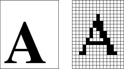
Computer software creates images on screen by writing data to memory locations in the frame buffer. To draw a pixel on screen, simply write an appropriate value in to the corresponding memory location, the pixel will then appear on screen during the next screen refresh. Because of the nature of raster displays, images, text, user-interface controls or anything that appears on screen must be converted into a set of discreet pixel values. This process is called rasterization, and usually produces a blocky approximation of the object being processed, with jagged edges. As long as the pixel size is small (high resolution), these effects are not noticeable. For low resolution displays, there are techniques (anti-aliasing) which reduce the appearance of jaggies, as in the figure below.

The number of colours supported by a device is usually referred to as the pixels bit-depth, as the number of bits used to store a pixels colour determines the number of possible colours for the pixel. 1 bit stores 2 colours (0=white, 1=black). Old EGA monitors had a bit depth of 4, which allowed 16 different colours. VGA monitors have a bit depth of 8, which allowed 256 colours. Modern monitors support up to 24 bit of colour information. Naturally, the larger the number of bits used for colour, the larger the amount of memory needed to store the image.
Devices, which use colour look-up tables(LUTs), can increase the number of colours available to images. These allow devices to display a larger range of colours than their bit-depth would normally allow. In an 8-bit system, a LUT is a table of 256 entries, each entry represents a colour and specifies the amount of red green and blue in the colour as an RGB triple. In the bit-map each pixel value represents an entry in the LUT. The bit-map would contain a header specifying the colours to be stored in the LUT. In this arrangement, a device can still only display 256 different colours (one for each entry in the table), but these colours can be selected to best match the image being displayed, e.g. if a forest scene was being displayed, the LUT may contain 100 different shades of green.
Line drawing is fundamental to computer graphics and it is important that the rasterization technique used for line drawing be as efficient as possible. In this section we will look at a highly efficient line drawing algorithm developed by Jack Bresenham. Lines are usually specified by giving start end and end points, A(a_{x},a_{y}) and B(b_{x},b_{y}). A line drawing algorithm then tries to turn on a set of pixels which approximates to an ideal line drawn between A and B. The equation of an ideal line is given as;
The slope of a line indicates how steep the line is, the actual value of the slope tells us how high the line rises, as x increases by one.
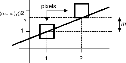
So, to determine the height of the line as we move across from one pixel to the next, simply add m to the current y-co-ordinate and round this value to get the current pixel position.
y=a.y;
for(x=a.x; x<=b.x; x++, y+=m)
    drawpixel(x,round(y));
This code will work, however y and m need to be
floats and floating point arithmetic (e.g. y+=m and
round(y)) is computationally very expensive. Bresenham was
able to refine the above algorithm to eliminate all floating point
arithmetic, thus giving us a very efficient line drawing method.
The algorithm calculates the position of the current pixel, by
using information about the position of the previous pixel. To
simplify matters, initially we will only consider lines with
slopes between 0 and 1( 0^{\circ} and 45^{\circ}). In this
restricted case, as x increases by one for each pixel, the
y co-ordinate of the next pixel either stays the same or
increases by one (figure below).

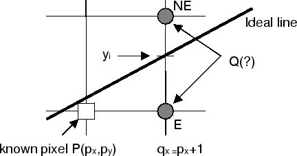
In figure above, the grid intersections represent the center of pixel positions. Assume we know the position of previous pixel P and are trying to determine the position of the current pixel Q. For lines with slopes between 0 and 1, Q will be at either E(q_{x},p_{y}) or at NE(q_{x},p_{y}+1). We will choose between E and NE by measuring the distance between these points and the y-value of the ideal line (y_{i});
Thus we increment the y co-ordinate if the above term is zero or positive and we don't increment if the term is negative.
The only non-integer in the above expression is m which we can rewrite as;
Now we can re-write the equation as;
We are only interested in the sign of this equation and not it's actual value, therefore, we can multiply across by \Delta x, because this will not change the sign. Therefore we get;
To determine if we should choose NE (increment y) or E (no change in y), simply evaluate the above expression (if it less than zero choose E).
We have removed the floating point components from the calculation, \Delta y=(b_{y}-a_{y}), \Delta x=(b_{x}-a_{x}) (all integers), but we still have expensive multiplication. Multiplication can be removed as follows;
Call the equation above e_{i} (expression for pixel i), the expression for the following pixel will be;
q_{y} is y co-ord for current pixel)
Note that (q_{y} - p_{y}) represents the difference in height between the y co-ords of the current pixel we've just drawn (Q) and the previous pixel (P). If there was no increment between P and Q, (q_{y} - p_{y}) will be 0 therefore;
So to evaluate the term for the next pixel, we only need the expression result for the current pixel e_{i} and the terms 2\Delta y and 2(\Delta y-\Delta x), which can be calculated quickly in advance using a bit-shift for the multiplication by 2. This method depends on knowing the result of previous pixel calculations. How do we start off?
The first pixel is placed at the point given as the start of the line A(ax,ay). The term for the second pixel can be calculated as;
Once we have a value for e_{i} we can quickly calculate the value of subsequent expressions; e_{i+1};
So our line drawing algorithim proceeds as follows;
Bresenham's Algorithm as described, only works for lines with slopes between 0 and 1 (case A). This limits us to drawing only \frac{1}{4} of all possible lines. We need to extend Bresenham's method to all lines.
There are two special cases of lines which can be drawn without Bresenham, horizontal (slope=0) and vertical lines (slope=\infty). For horizontal lines, simply increment the x co-ord, while keeping y constant. Vertical lines are drawn by keeping the x co-ord constant and incrementing y. These lines are appear quite frequently in applications, so it is worthwhile treating them differently. Note also, that lines with slopes of 1 and -1 can also be drawn very quickly (increment x and y together).
For lines with slopes greater than 1, interchange the roles of x and y. Increment y and test if the x co-ord needs changing (this basically turns the algorithm on its side). Lines with slope between 0 and -1 (case D), we run the algorithm as before, except that we use the test to determine when we should decrement the y co-ordinate. For Lines whose slope is less than -1, we can interchange the roles of x & y and decrement the x coordinate instead of incrementing.
So the final line drawing algorithm will first test if the requested line is one of the special cases outlined above, if not a special case \Delta x and $\Delta y are compared to see which 'version' of the algorithm should be applied.

Bresenham's line drawing algorithm can be used to draw lines with patterns; in figure above of patterned lines, the patterns are stored as sequences of 16 bits, this pattern is repeated over the length of the line. A line drawing algorithm to reproduce these lines would maintain a pointer into an array storing the pattern. This pointer would be incremented for each pixel position along the line. If the corresponding bit was 1, then a pixel would be drawn, otherwise no pixel is drawn and the algorithm would move onto the next pixel position. Once the pointer reached the end of the bit sequence, it should be reset to zero. A naïve algorithm would start a separate pattern for each line segment as in the box on the left of the figure , a new pattern is started for each edge, and this shows up as discontinuities at each corner. However, by maintaining a global (or preferably, static) pointer into the pattern sequence, the pattern can be continued between successive calls to the drawing algorithm (as long as the lines are drawn in order and start at the end point of the previous line). The pattern then appears to be continuous around the corners of a polygon (e.g. the box on the right of the figure).

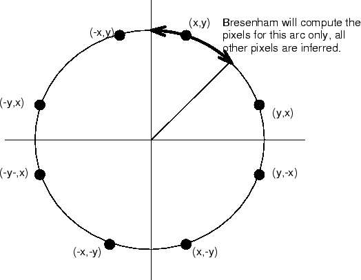
Initially, we will only consider a sub-set of the circle drawing problem and generalize it to the full circle later on. We will concentrate on the set of pixels representing the arc from 90^{\circ} to 45^{\circ} (figure below).
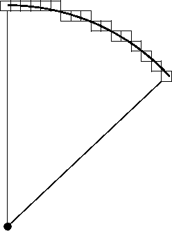
Starting from the left of figure and moving right along the arc, notice that each pixel along the arc of interest is either on the same level as the previous pixel or is moved down one-coordinate from the previous.
So for each pixel we have simple choice to make, choose the pixel to the East(E) of the previous pixel or to the South East (SE).
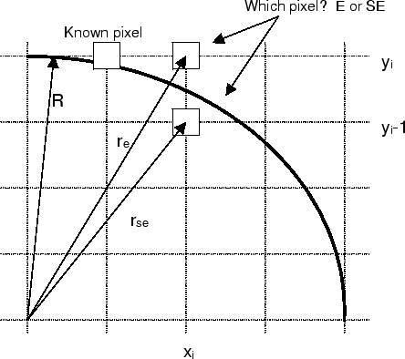
The approach now is similar to line drawing, we make our decision based on which pixel is nearest the ideal circle;
What remains is to manipulate the text above into a quickly calculable expression.
The algorithm proceeds by incrementing x for each new pixel and decrementing y only if e_{i} is greater than zero. Once the pixels for one octant have been calculated, it is a simple matter to generate the remaining pixels by reflection about the two axis and two diagonals.
© Ken Power 2010