Raytraced Image
Last Updated April 4, 2008
Rendering scenes using polygon meshes and shading techniques can produce realistic displays. Smooth shading techniques can remove the faceted nature of the meshes. However these methods are limited in the types of scenes that can be generated. Reflective surfaces and transparent materials cannot be rendered accurately. Shadows and 'Atmospheric' effects like fog or haze are difficult and expensive to implement.
Raytracing provides a powerful approach, which solves most of these problems. Although expensive, raytracing gives some of the most realistic results of any rendering technique. Instead of building a scene polygon by polygon, raytracing passes a ray from the eye through each pixel into the scene. The path of the ray is traced to see what object is strikes first and at what point (This automatically solves the hidden surface problem). From this point further rays are traced to all the light sources in the scene in order to determine how this point is illuminated. This determines if a point is in shadow. If the surface that has been struck is reflective and/or transparent, then further rays are cast in the direction of reflection or transmission. Then the contribution to surface shading of each of these rays is calculated. Each of these rays contributes to the eventual colour of the pixel.
Although raytracing can be applied to scenes modelled using polygon meshes, the most effective way to model scenes for raytracing purposes is Constructive Solid Geometry(CSG). CSG is the process of building solid objects from other solids. The three CSG operators are Union, Intersection, and Difference. Each operator acts upon two objects and produces a single object result. By combining multiple levels of CSG operators, complex objects can be produced from simple primitives. The union of two objects results in an object that encloses the space occupied by the two given objects. Intersection results in an object that encloses the space where the two given objects overlap. Difference is an order dependent operator; it results in the first given object minus the space where the second intersected the first.
A CSG system includes a number of primitive or generic objects from which complex scenes can be built. These objects usually include a unit sphere (centered on the origin, radius one), a unit cube, unit cone, unit cylinder, a plane etc. Transformations can be applied to these objects to rotate, scale (stretch) or twist (shear) by applying a transformation matrix. The transformations can be different in different axis, stretching a sphere along the x-axis produces an ellipsoid for example. When the primitive has been changed into the desired shape, it can be translated to a different position by adding a displacement vector. The resultant shapes can be combined using the CSG operators into compound objects. These compound objects can also be transformed and displaced and further combined. This process can created surprisingly complex and realistic models from a few simple building blocks. Each object or compound object can be given a number of properties, depending on the complexity of the raytracing engine. These include pigmentation, reflectivity, transparency and texture.
As with the synthetic camera process, a viewing co-ordinate system is defined, the position of the viewer (eye) is given and a viewport is defined on the viewing plane. The viewport is sub-divided by a grid of rows and columns, the number of which is determined by the required image resolution. Each square in this grid corresponds to one pixel on screen unless antialiasing is being used).
In the scene the position and properties (colour, intensity, shape etc) of light sources are specified. The objects in the scene are specified (usually) as a CSG model, the color, texture and other surface properties are also defined for the scene objects.
For each square (pixel) on the grid, a ray is built which extends from the eye through the centre of the square and into the scene. This ray is tested against all objects in the scene to determine which objects are intersected by the ray. This gives a list of points of intersection. The list is sorted and the intersection nearest the eye is determined. This point will be used for further processing. The colour returning from this point to the eye is calculated using an illumination model which takes into account the lights in the scene, the orientation of the surface and basic surface properties. This will be the final colour of the pixel. This is a simplified view of the process and these steps will produce images of the same quality as traditional mesh rendering.
To enhance realism a raytracer will cast secondary rays, which will add important details such as shadow, transparency and reflection to the scene.
A fundamental task in raytracing is determining where a ray intersects an object, this is usually the most expensive step so it is important that intersections be found as efficiently as possible. As we shall see, it can be relatively simple to find the intersection of a ray with one of the generic primitives (sphere, plane, cube etc). However, in CSG these primitives are usually subjected to a transformation and/or a translation. Objects transformed like this may have been scaled, rotated and sheared, this makes them very awkward to deal with in terms of finding intersections. To avoid this problem, we transform the ray and intersect it with the generic object.
A ray can be given as given as;
A transformation matrix, M, has been applied to our generic object and the object has been translated by d. So every point \vec{\mathbf{q}} on our primitive has been transformed to \vec{\mathbf{q'}};
Instead of intersecting \vec{\mathbf{r}}(t) with the transformed object \vec{\mathbf{q'}}, we will apply the reverse transformation to the ray by subtracting \vec{\mathbf{d}} and applying M^{-1}
A useful theorem from linear algebra tells us that if a ray, \vec{\mathbf{r}}(t), passes through a transformed point \vec{\mathbf{q'}}, at time t_{1}, then the transformed ray \vec{\mathbf{r'}}(t) passes through the point \vec{\mathbf{q}} at the same time, t_{1} (This assumes that the \mbox{$\vec{\mathbf{q}}$} \to \mbox{$\vec{\mathbf{q}}$}' transformation is the reverse of \mbox{$\vec{\mathbf{r}}$}\to \mbox{$\vec{\mathbf{r'}}$}). So, in order to find the point of intersection of a ray with an object, we reverse the transformation that created the object from a primitive and apply that reversed transformation to the ray. Then find the points of intersection of the transformed ray and the original primitive.
A generic sphere centered on the origin with a radius of 1 is given by;
squaring both sides:
Substitute a ray into this to determine intersections:
this can be written as the familiar quadratic at^{2}+bt+c=0 the solution of which is; \begin{displaymath} \frac{-b\pm\sqrt{b^{2}-4ac}}{2a} \end{displaymath}
The solutions to the quadratic give the time(s) of intersection. If this gives two real solutions, then the ray has intersected the sphere twice. If only one solution is found, then the ray is a tangent to the sphere. If no real solutions are found, then the ray does not intersect the sphere (if b^{2}<4ac, then there are no real solutions). Once the intersection times (hit times) are known, they can be inserted into the original equation of the ray to calculate the co-ordinates of intersection.
The generic plane is usually given as z=0 , a ray \mbox{$\vec{\mathbf{s}}$}+\mbox{$\vec{\mathbf{c}}$}t strikes this plane when its z-component is zero:
If c_{z} is zero then the ray is parallel with the plane and there is no intersection.
A generic square is a piece of the generic plane. First determine the co-ordinates of the ray intersecting the plane, and then test if the points' x and y co-ordinates lie outside the region of the square (usually 1\times 1 ).
To test for intersection with this cylinder, a test must first be made against the infinite cylinder lying along the z-axis. This is determined by substituting the ray \mbox{$\vec{\mathbf{s}}$}+\mbox{$\vec{\mathbf{c}}$}t into the equation for the cylinder x^{2}+y^{2}=1 (the x and y are replaced by the x and y components of the ray respectively). This gives a quadratic of the form At^{2}+2Bt+C=0 , which can be solved in the usuall method. If the solution(s) give hit time(s), with z-components between -1 and +1, then the ray hits the walls of the unit cylinder.
The ray may also strike the unit cylinder by piercing the caps. A test must be made to determine points of intersection with the planes z=-1 and z=1 , if the hit point lies within the radius of the cap ((s_{x}+c_{x}t_{h})^{2}+(s_{y}+c_{y}t_{h})^{2}\le1) , then the ray strikes the cylinder at that point.
The equation for an infinite double cone is $x^{2}+y^{2}=\frac{(1-z)^{2}}{4} , again hit points can be found by substituting x , y and z by the x, y, and z components of the ray and solving the resulting quadratic. Like the cylinder, the z co-ord of the hit points must occur between 0 and +1. Also a separate test must be made to determine if the base of the cone has been pierced.
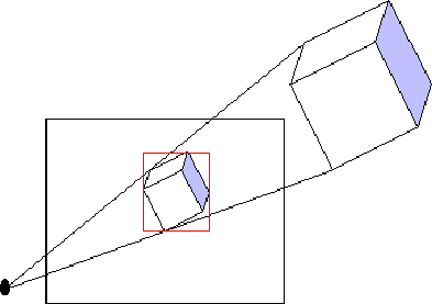
As has been seen, computing hit points for 3D objects can be expensive. If we have a scene with many objects, for each ray from the eye we need to check for intersections with all objects. However each ray will usually strike a small percentage of the objects in a scene. It has been estimated that 95% of the time of a naive raytracer is spent determining intersections. There would be a significant gain in efficiency if there was a way to quickly eliminate objects which are not struck by a given ray without having to perform the expensive tests seen above. This can be done by using extents. An extent defines a simple area around each object which can be quickly tested for intersections. For primary rays (rays from the eye), each object is projected onto the viewplane and the minimum bounding rectangle (MBR) for each object is calculated before raytracing begins). The MBR is determined by finding the maximum and minimum x and y co-ordinates for the projected image. Each ray is then tested to see if it intersects the MBR, (this is done by checking if this current pixel is inside the MBR), if it does not, the object cannot possibly be intersected by the ray and is ignored. If the MBR is intersected, we can then apply a more precise intersection test to determine if and where the ray intersects the object in question.
This process can be improved by using union extentsfor clusters of small objects. This involves finding a MBR which encloses a number of objects. Using union extents, large numbers of objects can be eliminated with one quick test.
A basic raytracer will compute the light intensity at a point, by using the surface normal, viewer and light orientation in an illumination model. But it is possible that a point is shaded from a light source by another object. This point is in shadow and there will be no diffuse or specular component from that light source.
To determine a if a point is in shadow with respect to a particular light source, a secondary ray is generated. This ray starts at the hit point on the surface in question ( t=0 ) and emanates to the light source ( t=1). This ray is then tested for intersections. If any intersections occur between t=0 and t=1, then the surface point is in shadow with respect to the objects intersected. This test is carried out for each of the light sources in the scene. Even is the scene contains only one object, a test for shadows must be carried out as an object can shadow itself. This process is a similar to testing the primary ray for intersections, except;
For a point on a surfaces which is reflective and/or transparent, the light returning to the eye will have 5 components:
\begin{displaymath} I_{tot}=I_{amb}+\underline{I_{diff}+ I_{spec}}+ I_{refl}+ I_{refr} \end{displaymath}The first three are familiar from the lighting model ( again there are separate diffuse and specular components for each light source, so the underlined component is repeated for each light source).
I_{refl} is the reflected light component. This is light arriving at the point along the direction of reflection.
The equation for this vector is;
\vec{\mathbf{b}}=\vec{\mathbf{dir}}-2(\vec{\mathbf{dir}}.\vec{\mathbf{N}})\vec{\mathbf{N}}
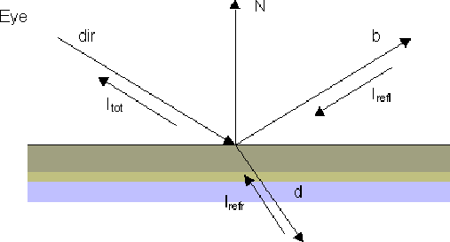
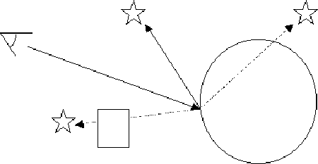
Similarly I_{refr} is the refracted component, which arises from light transmitted through the material along the direction -\mbox{$\vec{\mathbf{d}}$} . When light arrives at a material boundary it is "bent" continuing it's travel along vector -\mbox{$\vec{\mathbf{dir}}$} . Just as I_{tot} is a sum of various light contributions, I_{refl} and I_{refr} each arise from their own 5 components. These are computed by casting a secondary ray in the directions of reflection and refraction and then seeing what surface is hit first, the light components at that point are then computed, which in turn generates additional secondaries. In the figure below, I is the light arriving at the eye. It represents the sum of 3 components, reflected R_{1} ), transmitted ( T_{1} ) and the local component (not shown).
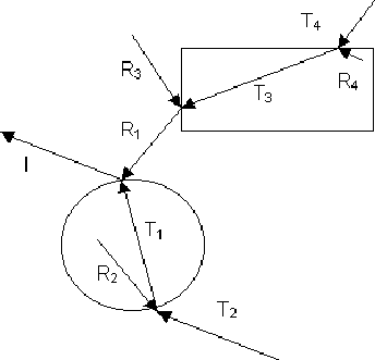
The local component is made up of ambient, diffuse and specular reflections. Each reflected component is in turn made up of three components, e.g. R_1 is composed of R_3 and $T_3 as well as the local components at that point. Each contribution is the sum of three others, this suggests a recursive approach to computing the light intensity. In principle, secondaries may be spawned ad-infinitum. However, in practice, raytracing usually spawns secondaries two levels deep, this limit may be locally increased for particularly reflective or transparent surfaces.
The refraction of light is determined by Snells law, which states that the sin of the angle of refraction \theta_2 is proportional to the sin of the angle of incidence \theta_1 .
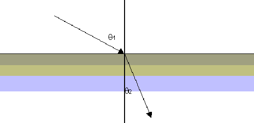
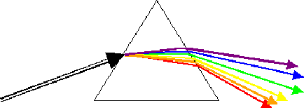
The constant of proportionality (n) is called the index of refraction. This value depends on the properties of the two materials through which the light is passing. Some useful values are; 1.33 for air-water and 1.60 for air-glass. This constant is slightly different for different wavelengths of light. For most materials the difference is insignificant. However, for materials like quartz, red light is refracted far more than green and blue light; this property causes rainbow effects.
However, some objects, are not suitable for sphere bounding, also, calculating the minimum bounding sphere can be difficult. A more useful general purpose bounding volume is the 6-sided box. The box is constructed with it's sides aligned with the co-ordinate axis, which allows intersections to be calculated efficiently. This box is built like the projection extent. The minimum and maximum x , y and z co-ordinate for all the vertices in the object are determined and these values from the sides of the box.
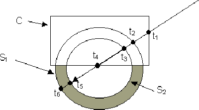
The ray in the diagram must pass through 4 intersections before first striking part of the surface of the bowl (t_5) . It is not possible to simply use the first intersection as in simple objects. In this case t_1 is the first intersection, but it does not form part of the visible surface. An intersection list must be build for each object; \begin{displaymath} S1(t_2,t_6), S2(t_3,t_5), C(t_1,t_4) \end{displaymath}
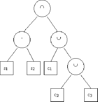
Because the CSG operators are binary, a natural data structure is a binary tree, where each node is an operator and each leaf is a primitive. e.g. (s1-s2)\cap(c1\cup c2\cup c3)
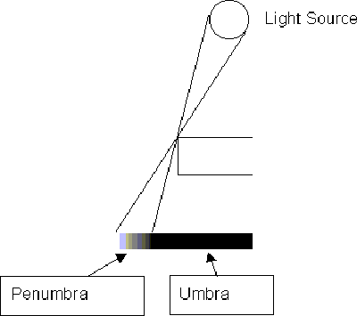
A simple raytracer assumes that traced rays are infinitely thin beams, this results in images with sharp shadows, sharp reflection and refraction, with everything in perfect focus. These artifacts lead to images having an easily identifiable computer generated signature.
Real surfaces do not reflect perfectly, reflections are slightly blurred because of small imperfections in the surface. For the same reason real materials do not transmit light perfectly. Shadows are never sharp because finite (real) light sources cause a penumbra shadow.
One approach to model these effects is distributed raytracing. This method typically an number of secondary rays (usually 16) for each primary ray. When each ray strikes a surface, it is not reflected or transmitted exactly in the predicted direction, instead the ray is cast in a random direction close to the predicted ray. How close the cast ray corresponds to the predicted ray depends on the surface properties. Similarly, when casting rays to determine shadow, the rays are not cast exactly in the direction of the light source, but to random points close to the light source. These 16 rays are averaged to determine the colour of that pixel.
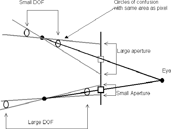
Traditional ray traced images typically have perfect focus throughout the scene. The human eye and cameras can only focus on a limited range in any given situation, this range is called the depth of field (DOF). The depth of field of an image depends on the aperture (width) of the lens. Wide lenses allow much light through, which is necessary for low light situations, but wide lenses have very small depth of field. The centre of the DOF is controlled by the focal length of the lens. The human eye can change both the aperture and focal length of its lens by widening the pupil or stretching the lens. Most cameras also have these features.
To achieve depth of field effects in raytracing, we must specify a focal plane, which is a plane parallel to the viewplane, this plane will be the centre of the required depth of field. All points on this plane will be in perfect focus. The focal plane is usually given as a distance from the viewplane (focal length). For each pixel, a primary ray is cast, the point at which this ray strikes the focal plane is called the focal point for this ray. An aperture value is given. This specifies the size of the region around the pixel from which further rays are cast, usually 4-16 additional rays. These rays are built so that they will intersect the focal point. Each of these rays are tested for intersections as normal and a colour is determined. The colour of the distributed rays is averaged and this colour is used for the pixel.
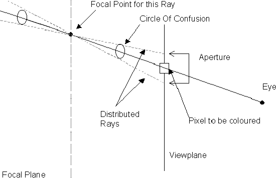
Notice that the distributed rays converge on the focal point. Before and after the focal point, the rays are spread over an area called the circle of confusion. This circle increases in size as the rays move away from the focal point. The size of the circle represents the area of the scene that is involved in producing the colour for a particular pixel. The larger this area is, then the more blurred the image becomes, because more components of the scene contribute to the colour at that pixel. There is region in which the circle of confusion is smaller than the resolution (pixel area), this is the depth of field. Parts of the scene in this area are in focus. Making the aperture smaller increases the depth of field .
© Ken Power 2009